Quickstart example

In the following example, we use the “test” MRIOT of the pymrio module, which doesn’t require loading additional data and has a low number of sectors and regions, allowing fast computation.

Instantiating a model from a MRIOT system

First import the required elements. We use the ARIOPsiModel version here (which you probably should as well).

# import pymrio for the test MRIOT
import pymrio

# import the different classes
from boario.extended_models import ARIOPsiModel  # The core of the model

Some attributes of the test MRIOT are not computed. Calling calc_all() ensures all required tables are present in the IOSystem object. This pymrio.IOSystem method automatically identifies which tables are missing and calculates them following the IO formal framework. (See here for more details.)

mriot = pymrio.load_test().calc_all()

If you see multiple: FutureWarning: DataFrame.groupby with axis=1 is deprecated. Do `frame.T.groupby(...)` without axis instead. don’t panic, this comes from pymrio but it is not an error, just a syntax warning.

In case you find it annoying, you can use the following beforehand:

import warnings

warnings.simplefilter(action="ignore", category=FutureWarning)

Instantiating the model is very straightforward:

model = ARIOPsiModel(mriot)

/home/sjuhel/Repos/BoARIO/boario/model_base.py:277: UserWarning: No capital to VA dictionary given, considering 4/1 ratio
  warnings.warn("No capital to VA dictionary given, considering 4/1 ratio")

This sets the model with all the default parameters. We highly recommand you to study the different parameters and their options for actual use. See Changing the model parameters.

By default, the model sets the productive capital of each industry to 4 times their Value Added (as Gross Ouptut - Intermediate Demand), you should not rely on this.

Similarly, instantiating a simulation is also quite easy:

from boario.simulation import Simulation  # Simulation wraps the model

sim = Simulation(model, n_temporal_units_to_sim=730)

Once the model and simulation have been instantiated, you can now define an event:

from boario import event

# Instantiate an event.
ev = event.from_scalar_regions_sectors(
    impact=5000000,
    event_monetary_factor=10**6,
    duration=15,
    event_type="rebuild",
    affected_regions=["reg1"],
    affected_sectors=["manufactoring", "mining"],
    impact_sectoral_distrib=model.mriot.x.loc["reg1", "indout"],
    impact_regional_distrib="equal",
    rebuilding_sectors={"construction": 0.55, "manufactoring": 0.45},
    rebuild_tau=180,
)

Here we define an event happening in region reg1 impacting the productive capital of the manufactoring [1] and mining sectors. The impact is distributed among the two sectors proportional to their production output (mriot.x).

Here the entire impact is translated into a reconstruction demand, handled by the construction (55%) and manufactoring (45%) sectors. This reconstruction has a characteristic time of 90 unit steps.

There are different types of Event subclasses implented in BoARIO, each with there specificities, to allow the modeling of different types of shocks. See Defining events, for more in depth explanation on how to define events.

[1]

This typo in the “manufacturing” sector’s name comes from pymrio.

The event can then be added to the simulation:

# Add the event to the simulation
sim.add_event(ev)

Note that by default, the impact is considered to be in single units of the currency, while often the MRIOTs are in Millions or Thousands. A warning is raised and the values are automatically adjusted accordingly. See Handling different monetary factors for more details.

And the loop can be run:

# Launch the simulation
sim.loop()

Once the simulation ran, you can access and plot the timeseries of the variables (see Monitoring the variables for a list of accessible variables).

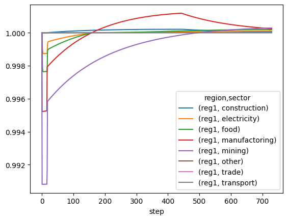
Here is an example showing the relative change in production in the different sectors in "reg1".

# You can generate a dataframe of
# the production with the following line
df = sim.production_realised
# This allows to normalize production at its initial level
df = df / df.loc[0]

df.loc[:, ("reg1", slice(None))].plot()

<Axes: xlabel='step'>